Kernel (image Processing) on:
[Wikipedia]
[Google]
[Amazon]
In
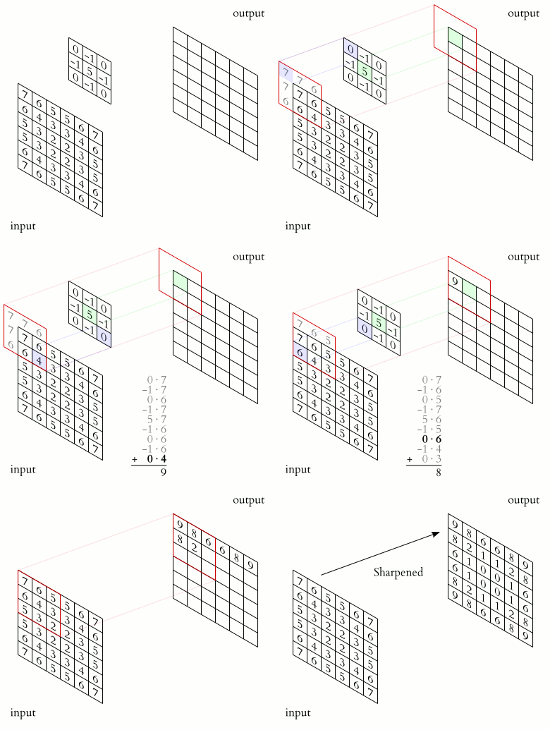
 Convolution is the process of adding each element of the image to its local neighbors, weighted by the kernel. This is related to a form of mathematical convolution. The matrix operation being performed—convolution—is not traditional matrix multiplication, despite being similarly denoted by *.
For example, if we have two three-by-three matrices, the first a kernel, and the second an image piece, convolution is the process of flipping both the rows and columns of the kernel and multiplying locally similar entries and summing. The element at coordinates , 2(that is, the central element) of the resulting image would be a weighted combination of all the entries of the image matrix, with weights given by the kernel:
The other entries would be similarly weighted, where we position the center of the kernel on each of the boundary points of the image, and compute a weighted sum.
The values of a given pixel in the output image are calculated by multiplying each kernel value by the corresponding input image pixel values. This can be described algorithmically with the following pseudo-code:
for each ''image row'' in ''input image'':
for each ''pixel'' in ''image row'':
set ''accumulator'' to zero
for each ''kernel row'' in ''kernel'':
for each ''element'' in ''kernel row'':
if ''element position'' corresponding* to ''pixel position'' then
multiply ''element value'' corresponding* to ''pixel value''
add ''result'' to ''accumulator''
endif
set ''output image pixel'' to ''accumulator''
:
Convolution is the process of adding each element of the image to its local neighbors, weighted by the kernel. This is related to a form of mathematical convolution. The matrix operation being performed—convolution—is not traditional matrix multiplication, despite being similarly denoted by *.
For example, if we have two three-by-three matrices, the first a kernel, and the second an image piece, convolution is the process of flipping both the rows and columns of the kernel and multiplying locally similar entries and summing. The element at coordinates , 2(that is, the central element) of the resulting image would be a weighted combination of all the entries of the image matrix, with weights given by the kernel:
The other entries would be similarly weighted, where we position the center of the kernel on each of the boundary points of the image, and compute a weighted sum.
The values of a given pixel in the output image are calculated by multiplying each kernel value by the corresponding input image pixel values. This can be described algorithmically with the following pseudo-code:
for each ''image row'' in ''input image'':
for each ''pixel'' in ''image row'':
set ''accumulator'' to zero
for each ''kernel row'' in ''kernel'':
for each ''element'' in ''kernel row'':
if ''element position'' corresponding* to ''pixel position'' then
multiply ''element value'' corresponding* to ''pixel value''
add ''result'' to ''accumulator''
endif
set ''output image pixel'' to ''accumulator''
:* corresponding input image pixels are found relative to the kernel's origin.
If the kernel is symmetric then place the center (origin) of the kernel on the current pixel. The kernel will overlap the neighboring pixels around the origin. Each kernel element should be multiplied with the pixel value it overlaps with and all of the obtained values should be summed. This resultant sum will be the new value for the current pixel currently overlapped with the center of the kernel.
If the kernel is not symmetric, it has to be flipped both around its horizontal and vertical axis before calculating the convolution as above.
The general form for matrix convolution is
 Kernel convolution usually requires values from pixels outside of the image boundaries. There are a variety of methods for handling image edges.
; Extend
: The nearest border pixels are conceptually extended as far as necessary to provide values for the convolution. Corner pixels are extended in 90° wedges. Other edge pixels are extended in lines.
; Wrap
:The image is conceptually wrapped (or tiled) and values are taken from the opposite edge or corner.
; Mirror
: The image is conceptually mirrored at the edges. For example, attempting to read a pixel 3 units outside an edge reads one 3 units inside the edge instead.
; Crop / Avoid overlap
: Any pixel in the output image which would require values from beyond the edge is skipped. This method can result in the output image being slightly smaller, with the edges having been cropped. Move kernel so that values from outside of image is never required. Machine learning mainly uses this approach. Example: Kernel size 10x10, image size 32x32, result image is 23x23.
; Kernel Crop
: Any pixel in the kernel that extends past the input image isn't used and the normalizing is adjusted to compensate.
; Constant
: Use constant value for pixels outside of image. Usually black or sometimes gray is used. Generally this depends on application.
// author : csblo
// Work made just by consulting :
// https://en.wikipedia.org/wiki/Kernel_(image_processing)
// Define kernels
#define identity mat3(0, 0, 0, 0, 1, 0, 0, 0, 0)
#define edge0 mat3(1, 0, -1, 0, 0, 0, -1, 0, 1)
#define edge1 mat3(0, 1, 0, 1, -4, 1, 0, 1, 0)
#define edge2 mat3(-1, -1, -1, -1, 8, -1, -1, -1, -1)
#define sharpen mat3(0, -1, 0, -1, 5, -1, 0, -1, 0)
#define box_blur mat3(1, 1, 1, 1, 1, 1, 1, 1, 1) * 0.1111
#define gaussian_blur mat3(1, 2, 1, 2, 4, 2, 1, 2, 1) * 0.0625
#define emboss mat3(-2, -1, 0, -1, 1, 1, 0, 1, 2)
// Find coordinate of matrix element from index
vec2 kpos(int index)
// Extract region of dimension 3x3 from sampler centered in uv
// sampler : texture sampler
// uv : current coordinates on sampler
// return : an array of mat3, each index corresponding with a color channel
mat3 region3x3(sampler2D sampler, vec2 uv)
// Convolve a texture with kernel
// kernel : kernel used for convolution
// sampler : texture sampler
// uv : current coordinates on sampler
vec3 convolution(mat3 kernel, sampler2D sampler, vec2 uv)
void mainImage( out vec4 fragColor, in vec2 fragCoord )
Implementing 2d convolution on FPGA
* ttps://www.shadertoy.com/view/3sGXWh GLSL Demonstration of 3x3 Convolution Kernels
Complete C++ open source project
Image processing Feature detection (computer vision) Articles with example pseudocode
image processing
An image or picture is a visual representation. An image can be two-dimensional, such as a drawing, painting, or photograph, or three-dimensional, such as a carving or sculpture. Images may be displayed through other media, including a pr ...
, a kernel, convolution matrix, or mask is a small matrix used for blurring, sharpening, embossing, edge detection, and more. This is accomplished by doing a convolution
In mathematics (in particular, functional analysis), convolution is a operation (mathematics), mathematical operation on two function (mathematics), functions f and g that produces a third function f*g, as the integral of the product of the two ...
between the kernel and an image
An image or picture is a visual representation. An image can be Two-dimensional space, two-dimensional, such as a drawing, painting, or photograph, or Three-dimensional space, three-dimensional, such as a carving or sculpture. Images may be di ...
. Or more simply, when each pixel in the output image is a function of the nearby pixels (including itself) in the input image, the kernel is that function.
Details
The general expression of a convolution is where is the filtered image, is the original image, is the filter kernel. Every element of the filter kernel is considered by and . Depending on the element values, a kernel can cause a wide range of effects: The above are just a few examples of effects achievable by convolving kernels and images.Origin
The origin is the position of the kernel which is above (conceptually) the current output pixel. This could be outside of the actual kernel, though usually it corresponds to one of the kernel elements. For a symmetric kernel, the origin is usually the center element.Convolution
 Convolution is the process of adding each element of the image to its local neighbors, weighted by the kernel. This is related to a form of mathematical convolution. The matrix operation being performed—convolution—is not traditional matrix multiplication, despite being similarly denoted by *.
For example, if we have two three-by-three matrices, the first a kernel, and the second an image piece, convolution is the process of flipping both the rows and columns of the kernel and multiplying locally similar entries and summing. The element at coordinates , 2(that is, the central element) of the resulting image would be a weighted combination of all the entries of the image matrix, with weights given by the kernel:
The other entries would be similarly weighted, where we position the center of the kernel on each of the boundary points of the image, and compute a weighted sum.
The values of a given pixel in the output image are calculated by multiplying each kernel value by the corresponding input image pixel values. This can be described algorithmically with the following pseudo-code:
for each ''image row'' in ''input image'':
for each ''pixel'' in ''image row'':
set ''accumulator'' to zero
for each ''kernel row'' in ''kernel'':
for each ''element'' in ''kernel row'':
if ''element position'' corresponding* to ''pixel position'' then
multiply ''element value'' corresponding* to ''pixel value''
add ''result'' to ''accumulator''
endif
set ''output image pixel'' to ''accumulator''
:
Convolution is the process of adding each element of the image to its local neighbors, weighted by the kernel. This is related to a form of mathematical convolution. The matrix operation being performed—convolution—is not traditional matrix multiplication, despite being similarly denoted by *.
For example, if we have two three-by-three matrices, the first a kernel, and the second an image piece, convolution is the process of flipping both the rows and columns of the kernel and multiplying locally similar entries and summing. The element at coordinates , 2(that is, the central element) of the resulting image would be a weighted combination of all the entries of the image matrix, with weights given by the kernel:
The other entries would be similarly weighted, where we position the center of the kernel on each of the boundary points of the image, and compute a weighted sum.
The values of a given pixel in the output image are calculated by multiplying each kernel value by the corresponding input image pixel values. This can be described algorithmically with the following pseudo-code:
for each ''image row'' in ''input image'':
for each ''pixel'' in ''image row'':
set ''accumulator'' to zero
for each ''kernel row'' in ''kernel'':
for each ''element'' in ''kernel row'':
if ''element position'' corresponding* to ''pixel position'' then
multiply ''element value'' corresponding* to ''pixel value''
add ''result'' to ''accumulator''
endif
set ''output image pixel'' to ''accumulator''
:Edge handling
 Kernel convolution usually requires values from pixels outside of the image boundaries. There are a variety of methods for handling image edges.
; Extend
: The nearest border pixels are conceptually extended as far as necessary to provide values for the convolution. Corner pixels are extended in 90° wedges. Other edge pixels are extended in lines.
; Wrap
:The image is conceptually wrapped (or tiled) and values are taken from the opposite edge or corner.
; Mirror
: The image is conceptually mirrored at the edges. For example, attempting to read a pixel 3 units outside an edge reads one 3 units inside the edge instead.
; Crop / Avoid overlap
: Any pixel in the output image which would require values from beyond the edge is skipped. This method can result in the output image being slightly smaller, with the edges having been cropped. Move kernel so that values from outside of image is never required. Machine learning mainly uses this approach. Example: Kernel size 10x10, image size 32x32, result image is 23x23.
; Kernel Crop
: Any pixel in the kernel that extends past the input image isn't used and the normalizing is adjusted to compensate.
; Constant
: Use constant value for pixels outside of image. Usually black or sometimes gray is used. Generally this depends on application.
Normalization
Normalization is defined as the division of each element in the kernel by the sum of all kernel elements, so that the sum of the elements of a normalized kernel is unity. This will ensure the average pixel in the modified image is as bright as the average pixel in the original image.Optimization
Fast convolution algorithms include: * separable convolutionSeparable convolution
2D convolution with an ''M'' × ''N'' kernel requires ''M'' × ''N'' multiplications for each sample (pixel). If the kernel is separable, then the computation can be reduced to ''M'' + ''N'' multiplications. Using separable convolutions can significantly decrease the computation by doing 1D convolution twice instead of one 2D convolution.Implementation
Here a concrete convolution implementation done with the GLSL shading language :See also
* Convolution in mathematics * Multidimensional discrete convolutionReferences
Sources
* * * * {{cite book , last2= Stockman , first2= George C. , last1= Shapiro , first1= Linda G., author1-link=Linda Shapiro , date= February 2001 , title= Computer Vision , pages= 53–54 , publisher= Prentice Hall , isbn= 978-0130307965External links
Implementing 2d convolution on FPGA
* ttps://www.shadertoy.com/view/3sGXWh GLSL Demonstration of 3x3 Convolution Kernels
Complete C++ open source project
Image processing Feature detection (computer vision) Articles with example pseudocode